The meaning of median

Or, how I learned to stop worrying and love the median.

Somewhere in school, we learn about the mean (aka the average, or the arithmetic mean) – add up a bunch of numbers and divide by how many there are. If you need to represent a bunch of numbers by one number, the mean is not a bad choice. The mean has desirable properties, in that it’s easy to compute incrementally – by keeping a running total and count, and it’s good for predicting aggregate behaviour – the total income tax collected by a government is the average income tax collected per person multiplied by the number of people.

We also learn about the median – sort a bunch of numbers into ascending order, and pick the middle one. This definition always struck me as a weird thing as a kid – it’s so unmathsy. The middle one? Where are the operations like sum and divide? What if there are an even number of data points – which one is the middle? It’s a pain to compute – you need to keep lots of data around. Later in life I came to appreciate that the median was really useful for predicting typical behaviour – the median income is a good estimate of the typical income of one person – it is much more resistant to outliers.

This post is about another way to think about the median which hopefully makes it seem more mathsy, illuminates why it is outlier resistant, and illustrates one of the ways that abstractions help connect distant parts of mathematics.

So tell me again about the mean?

Why is the mean a good estimate? What is special about \((a_1+...+a_n)/n\)?

To start, let’s think just about two numbers – \(a\) and \(b\) – and think of them as a point in the plane \((a,b)\). Say you want to estimate this with one number \(x\). That is, you want to pick \(x\) so that the point \((x,x)\) is as close as possible to the point \((a,b)\). What does close mean in the plane?

Our old friend Pythagoras has a theorem for that – the distance \(D\) is given by

\[ D = \sqrt{(x-a)^2 + (x-b)^2}. \]

To get as close as possible, we want \(D\) to be as small as possible. The smallest square root happens when the argument is as small as possible. How small can we make the error

\[ e(x) = (x-a)^2 + (x-b)^2 \]

by varying \(x\)? You might recall from calculus that our old friends Leibniz and Newtown figured out you could do this using differential calculus. The technique is to differentiate with respect to \(x\)

\[ e'(x) = 2(x-a) + 2(x-b) \]

and set equal to this equal zero, and solve:

\[ \begin{eqnarray} 2(x-a) + 2(x-b) &=& 0 \\ (x-a) + (x-b) &=& 0 \\ 2x &=& a + b \\ x &=& (a + b)/2 \end{eqnarray} \]

Hey presto – it’s the mean!

The same trick works with \(n\) points \(a_1,...,a_n\) – the single value \(x\) that makes the distance from \((x,...,x)\) to \((a_1,...,a_n)\) as small as possible needs to minimise the square error

\[ e(x) = (x-a_1)^2 + ... + (x-a_n)^2 \]

which happens when the derivative

\[ e'(x) = 2(x-a_1) + ... + 2(x-a_n) \]

is zero, that is, when

\[ \begin{eqnarray} 2(x-a_1) + ... + 2(x-a_n) &=& 0 \\ (x-a_1) + ... + (x-a_n) &=& 0 \\ nx &=& a_1 + ... + a_n \\ x &=& (a_1 + ... + a_n)/n \\ \end{eqnarray} \]

I really like this – when I learnt about the mean in school, it was like a law of nature – the formula as handed down by inscrutable ancients. The above shows why this is a good formula – it is the best single value approximating a set of numbers, where by best we mean “minimising the distance” between the \(n\)-tuples.

I thought this was about the median?

The above definition doesn’t appear to have much we can change about it – find a single \(x\) so that \((x,...,x)\) is as close as possible to \((a_1,...,a_n)\)? However, there is one thing we can change – the meaning of close! What could close mean? What if we are flexible in our understanding of distance?

Imagine that you could only move parallel to the axes. You can move up and down, or left and right, but not diagonally. You can still get everywhere, it just takes a little longer. This is called the Manhattan metric, because it’s like being trapped in a city where the streets make a grid and you can’t cut corners. What does distance mean here?

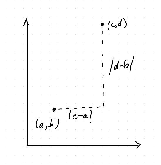
In this world, the distance from \((a,b)\) to \((c,d)\) is \(|c-a|+|d-b|\) – the sum of the absolute values of the differences in the coordinates. The absolute values are here because it doesn’t matter if you go left or right. You can do the same thing for \(n\)-tuples also – the distance from \((a_1,...,a_n)\) to \((c_1,...,c_n)\) is \(|c_1-a_1|+...+|c_n-a_n|\).

Now let’s take a look at the distance from \((a,b)\) to \((x,x)\) – it’s

\[ e(x) = |x-a|+|x-b| \]

We want to minimize this error. I find this easiest to understand by looking at its graph:

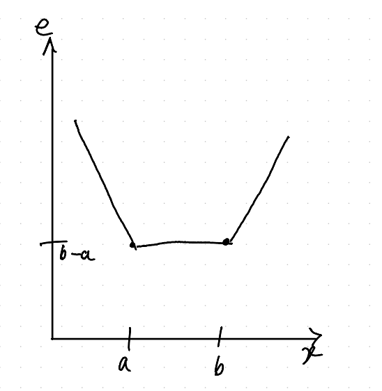
Note that I’ve drawn it for \(a < b\), the same thing happens in reverse if they’re the other way around.

Imagine sliding \(x\) along the \(x\)-axis from left to right. As long as \(x\leq a < b\), then \(|x-b|=|x-a|+|b-a|\) because you need to go through \(a\) to get to \(b\) from \(x\), and this means that

\[ |x-a|+|x-b|=2|x-a|+|b-a| \]

which explains the leftmost down slope.

For \(a\leq x\leq b\), the error \(|x-a|+|x-b|\) is constant – you pay once for the space between \(a\) and \(x\), and once for the space between \(x\) and \(b\), for a total of \(|b-a|\).

Once For \(a < b\leq x\), it slopes up again using the first argument in reverse.

So the closest you can get is for any \(x\) between \(a\) and \(b\) – which all result in the same error.

If you have three values \(a\), \(b\), and \(c\), something similar happens, but it’s a bit clearer maybe:

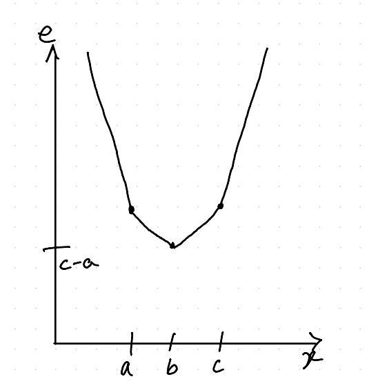
Far to the left, \(|x-b|=|x-a|+|b-a|\) and \(|x-c|=|x-a|+|c-a|\), so

\[ |x-a| + |x-b| + |x-c|= 3|x-a| + |b-a| + |c-a| \]

which explains the slope down as \(x\) approaches \(a\). Once \(x\) is between \(a\) and \(c\), we see that \(|x-a|+|x-c|=|c-a|\) because there’s no overlap, and so

\[ |x -a| + |x-b| + |x-c|= |x-b| + |c-a| \]

which explains the slope down as \(x\) approaches \(b\). Similarly, the graph slopes up after we pass \(b\), getting steeper as we pass \(c\). Notice when the error is smallest – it is when \(x=b\) – the median!

So the best Manhattan metric approximation to \((a,b,c)\) by a point like \((x,x,x)\) is to choose \(x\) to be the median value.

If you add more points, the same pattern happens. Sort the points into ascending order \((a_1,...,a_n)\) and consider the error \(|x-a_1|+...+|x-a_n|\).

Once \(x\) is between \(a_1\) and \(a_n\) their joint contribution becomes constant \(|a_n-a_1|\), whereas outside this interval the distance from \(x\) to the nearer endpoint contributes twice in addition. Similarly \(a_2\) and \(a_{n-1}\), and so on. This continues until either you find a minimum at the middle point \(a_{(n-1)/2}\) (if \(n\) is odd), or over the range \(a_{n/2}\) to \(a_{(n/2)+1}\) (if \(n\) is even). Conventionally we take the mean of the centre two points in the even case, but from this perspective, any value in that range is as good as any other.

In other words, the median is the closest single value approximation to an \(n\)-tuple using the Manhattan metric. When I found this out, I was astonished. The median is perfectly mathsy if you look at it right. In fact it’s even exactly the same definition as the mean, but just for a different meaning of distance.

And what about the outliers?

One of the useful things about the median is that it is resistant to outliers. To use the example from above, the average income is changed noticeably if you add a smaller number of much higher income people to the population. The median, on the other hand, is not significantly affected. This makes the median a much better measure if your goal is to understand “the typical experience”.

I’ll try to guide your intuition about why this is true. What we learnt above was that

• Mean – the closest single value approximation to an \(n\)-tuple using ordinary distance
• Median – the closest single value approximation to an \(n\)-tuple using manhattan distance

Now think about the value of \(\sqrt{a^2 + b^2}\) when \(a\) and \(b\) are very different in size. Squaring a big number makes it bigger faster than squaring a small number. So by squaring before we add, we increase the impact of the big number. If \(b\) is 10 times \(a\), then \(b^2\) is 100 times \(a^2\), and so its more important to get the big numbers right to minimise the error.

The same thing happens for \(\sqrt{(x-a_1)^2 + ... + (x-a_n)^2}\) – the largest terms get a boost because we square everything before adding, so \(x\) needs to be closer to the larger values.

By contrast, \(|a_1|+...+|a_n|\) has no such boost. Changing any number changes the total by the same amount. Consequently, the median, which is minimising \(|x-a_1|+...+|x-a_n|\) – a distance which doesn’t boost the large terms – is more outlier resistant.

You can just change what distance means?

One of the really powerful facets of mathematics lies in abstraction. By recognising what really matters in a situation, everything else can be flexible, and we can find new applications of tools that we know. Sometimes two concepts which look very different on the surface, are actually exactly the same concept once you find the right abstraction. The example in this post – mean and median – is just one example of this.

When you abstract something in maths, you don’t throw everything away. With nothing to start with, you can’t prove any theorems. In this example, we’re abstracting distance by abstracting to a metric. A metric assigns to each pair of points \(P\) and \(Q\) a non-negative distance \(D(P,Q)\) between them satisfying three axioms, which are, in both maths and intuitive forms:

1. \(D(P,Q)=0\) if, and only if, \(P=Q\)

   Different points are not in the same place

2. \(D(P,Q)=D(Q,P)\)

   The distance there is the same as the distance back

3. \(D(P,Q)\leq D(P,R)+D(R,Q)\)

   You can’t get somewhere quicker by going to more places

The last of these is also called the triangle inequality, and it captures the intuition that “the shortest path is a straight line” . Once you have these properties, you can do lots of mathematics with metrics. Both the ordinary distance (also known as Euclidean distance) and the Manhattan distance above satisfy all three of these properties, as do many other things.

I like to think of axioms like this as the APIs of mathematics – or maybe its closer to say I think of APIs as the axioms of systems. We find abstractions which hide details, but still provide enough power to let us use them to solve multiple different problems.